Hi everyone. In the last Friday challenge, we had a user post this question about an Excel Column Chart:
Chart: Remove whitespace from empty (non-existent) columns
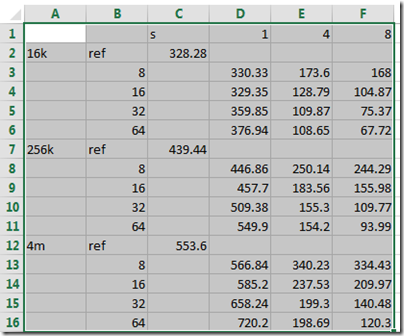
I’m trying to generate a graph from this table.
Excel 2012
| A | B | C | D | E | F | |
|---|---|---|---|---|---|---|
| 1 | s | 1 | 4 | 8 | ||
| 2 | 16k | ref | 328.28 | |||
| 3 | 8 | 330.33 | 173.6 | 168 | ||
| 4 | 16 | 329.35 | 128.79 | 104.87 | ||
| 5 | 32 | 359.85 | 109.87 | 75.37 | ||
| 6 | 64 | 376.94 | 108.65 | 67.72 | ||
| 7 | 256k | ref | 439.44 | |||
| 8 | 8 | 446.86 | 250.14 | 244.29 | ||
| 9 | 16 | 457.7 | 183.56 | 155.98 | ||
| 10 | 32 | 509.38 | 155.3 | 109.77 | ||
| 11 | 64 | 549.9 | 154.2 | 93.99 | ||
| 12 | 4m | ref | 553.6 | |||
| 13 | 8 | 566.84 | 340.23 | 334.43 | ||
| 14 | 16 | 585.2 | 237.53 | 209.97 | ||
| 15 | 32 | 658.24 | 199.3 | 140.48 | ||
| 16 | 64 | 720.2 | 198.69 | 120.3 |
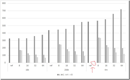
It turns out like this. 
This is almost what I need however there is an unnecessary whitespace for every blank cell. It’s more obvious when you look at the ref bars. I suppose Excel is creating a column of height 0 for every blank cell. I really need to change this behavior and remove those empty columns. Can somebody help me?
Well I received a few responses. But one was the best.
Don showed me the easiest way to solve this problem. To be frankly honest, I was way way over complicating this issue for the user by totally rearranging the data. However, this particular data set is custom made to Don’s solution and what I was thinking of would work in more complicated situations. So lets cover Don’s easy solution. I will post a Part 2 with a more complicated data set in a future Friday Challenge.
The Breakdown
1) Create Excel 2D Clustered Column Chart
2) Move the “ref” column to the 2nd axis
Step-by-Step
1) Create Excel 2D Clustered Column Chart
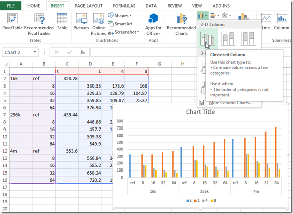
Select the data range from A1:F16
Select the 2-D Clustered Column Chart from the Insert Ribbon under the Charts Grou![]()

2) Move the “ref” column to the 2nd axis
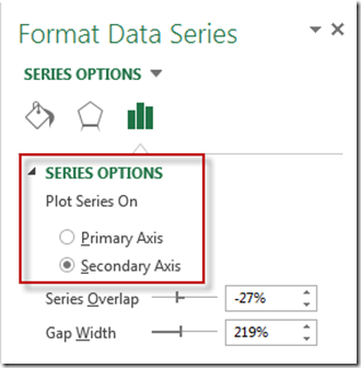
Select the chart and then select the “ref” column data series (the blue one if you are not color blind). Then press CTRL+F1 keys to bring up the Format Data Series dialog box and menu. Then choose the Secondary Axis radio button to move the series to the secondary axis. 
It will now be centered and will appear to remove the white space. All Done. Very simple, very easy!
I really thought it was going to be harder than that. I guess I should have looked at the data and also gave it a try. WAY TO GO DON!!
Video Tutorial
Free Excel Chart Template File Download: Remove-White-Space-Part-1.xlsx
Steve=True


