Add a Target Line to an Excel Pivot Chart

Many Excel users use Pivot Tables and they find it very easy to create a Pivot Chart.  However, Pivot Charts have some limitations.  For instance, Pivot Chart series must be part of the Pivot Table.  So that being said, many users find it difficult to understand how they can add a Goal or Target line to their Pivot Chart.

In this tutorial, I will show you the three ways that you can add a target or goal line to an Excel Pivot Chart.

1) Draw a Goal Line Using Excel Shapes

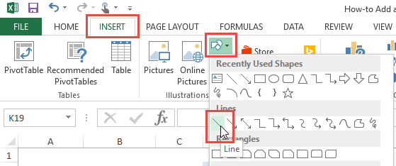
The first way to add a target threshold to an Excel Pivot Chart is the most simplest, but has the most inherent problems.  The easiest way that I am sure you already figured out is to draw a line with the Shapes feature in Excel Illustrations under the Insert Ribbon.

There are several issues with this approach.

a) Your data may change and the line will no longer be at the right threshold level.

b) If you move or resize your chart, the line may not move along with it.

c) You may not put the line at the correct chart data point.

d) It can be tough to draw a straight line with your mouse.  Now this one I solved in a recent post.  You can check it out here:

How to draw a straight line with Excel shapes

2) Add Data Series to Your Pivot Table

The next method that you can use is to modify your data set.  In order to do this, you will need to include additional data to your original data set that will represent the data for the Excel goal line.  It is relatively easy, in that, you need to add a new column of data to your original data set for the Pivot Table.

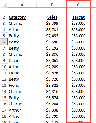
To do this, add a new column of data to your original data.  In our case, since it is a horizontal line, we would add the same value across the entire data range.  Then create your Pivot Table and include the additional column of data.

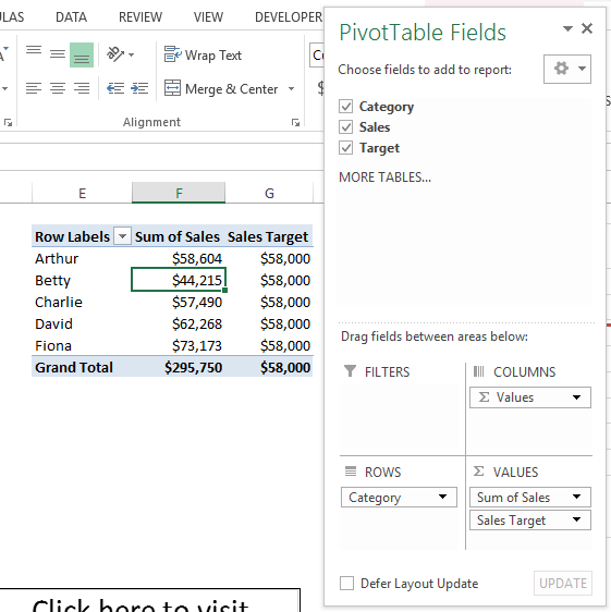
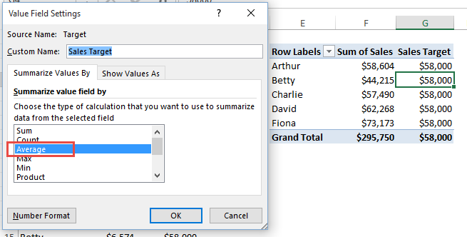
However, you need to summarize this new column of data as average (as the average across the range will be equal to the value in the column of target data).

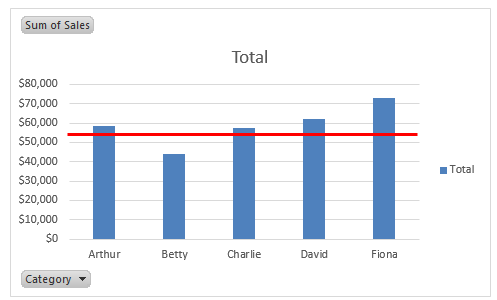
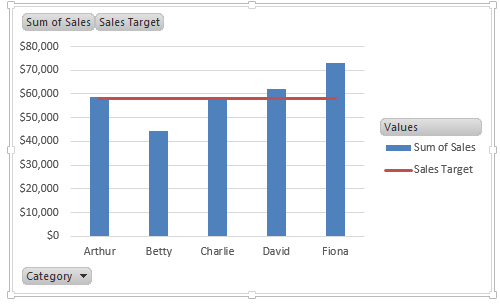
When you create your chart with the new sales target data point as part of the pivot chart, you will not have to worry about the previous issues you had with the drawn line.  However, you have added many new data points to your data set that will add size the to the Excel file.  For small data sets, this is not a problem, but if you have thousands and thousands of rows, this will add considerable size to your Excel file.  Although, your target threshold line will be in the right place and it will move and size with the Pivot Chart.

3) Create an Excel Pivot Table Calculated Field

This is the option that I would normally choose when adding a Goal Line to a Pivot Chart.  That being that you would create a calculated field in your Pivot Table and then add that to your Pivot Chart.  In order to do this, you should check out this post:

How-to create modify and delete an Excel pivot table calculated field

Since our scenario is to add a target line to the Pivot Chart, you will simply add a calculated field equal to a set value to your Pivot Table.

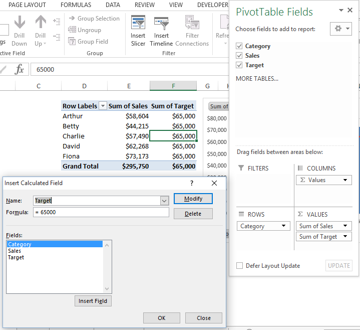
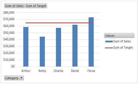
Since it is a calculated field in the Pivot Table, it doesn’t matter if you Average or Sum the Pivot Table Field as the final value will be the same that you desire for the Pivot Chart Target Line.

Hopefully this will help you quickly and easily add a goal/target/threshold line to your Pivot Charts.

Video Demonstration:

Sample File Download

How-to-Add-a-Goal-Line-or-Target-Threshold-to-an-Excel-Pivot-Chart.xlsx

What other tips and tricks to you have about Pivot Tables and Pivot Charts?  Let me know your favorite in the comments below.

Steve=True