There are many ways to Sum data in Excel. But when you have lots and lots of data, then you will want to learn a few different techniques. In our last post, you were presented with a challenge of summing 150,000 data points in several ways. One is a SumProduct formula, one was a SumIFS formula and one was to do it as quickly as possible using a Pivot Table. If you want to download the data and try it for yourself, go to this post: Friday Challenge – Advanced Excel Summation Skills
So that we can check out work on the other advanced Excel formula techniques, we should first create the Pivot Table version so that we know is the right answer. Some may call this a Check Sum to validate our answers for the SumProduct and SumIFS formulas.

Normally, I would have added 2 more columns of data to the spreadsheet data. I would have created one column for month of the transaction date and one for year. Then I would use those new data points as my columns and filters. However, this will make your file a lot larger when you are talking about 150,000 data points. So this is not highly desirable. Therefore, we should learn some more advanced Excel Pivot Table Options.
The Breakdown
1) Create Pivot Table
2) Create Group on Date
3) Filter Dates
Step-by-Step
1) Create Pivot Table
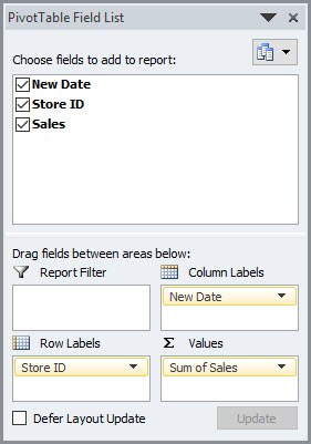
First, we need to create the Pivot Table by highlighting all 150,000 data points including the header labels and then go to your Insert Ribbon and Click on Pivot Table. It doesn’t matter where you put it (i.e. on a new sheet or existing sheet, just don’t put it directly on top of the data. Then, put “New Date” in the Columns, then put “Store ID” into the Rows and put “Sales into the Values section of the Pivot Table Field List.
Your Pivot Table Field List will look like this when you are done:
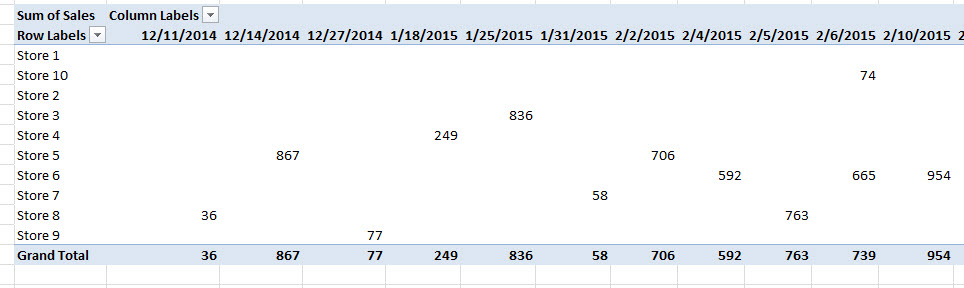
Your Pivot Table results will look like this:
2) Create Group on Date
Now that we have our Pivot Table created, we need to create some groupings. I will show you the technique I like but I also show you another way in the Video. It is a short video, show check it out below.
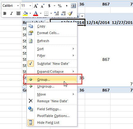
To create our Groupings for the Pivot Table, first Right Click on one of any of the dates that you see in the various columns. You will then see this pop-up menu:
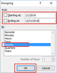
Next, you will see this Excel Pivot Table Grouping Dialog Box. From here, you will want to enter in the Start Date of 1/1/2016 and an End Date of 12/31/2016. Also, choose “By” as Months and click on the Okay button.
Once you click on okay, your Pivot Table results will change and look as you see here:
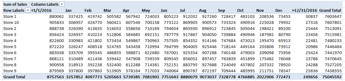
You will notice that the Pivot Table is now Grouped on data for months with anything before the start date that we entered under <1/1/2016 and anything after our end date showing up under >12/31/2016. We will filter these out in our next steps, but you can see that Excel’s Pivot Table Grouping feature is very powerful.
3) Filter Dates
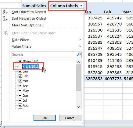
To Filter out the dates that we don’t want (before January 2016 and in 2017 and beyond), we need to simply click on the Sort and Filter Pull Down Options on the Column Labels in the Pivot Table. Then uncheck the “<1/1/2016” value and also uncheck the “>12/31/2016” values in the filter list.
Your final Sales Data Pivot Table by Store by Month for 2016 will look like this:
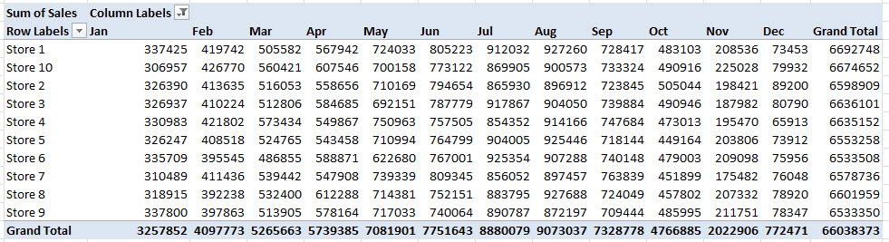
That was a lot simpler than what I used to do. We can also use this for the Check Sum against our SumProduct and SumIFS functions/formulas that I will show you in the next several videos. And finally, I will show you an Array solution as bonus material as well.
Video Demonstration
Check out a video tutorial of this Excel Tip and also the additional way you can do Pivot Table Groupings.
Were you able to do it with a Pivot Table in another fashion? If so, let me know how you did it using Pivot Tables in the comments below.
Steve=True


